SSCWeb Quick Start Guide
Table of Contents
1. Introduction
The Satellite Situation Center (SSCWeb) is a system run by the Space Physics Data Facility (SPDF) at NASA/GSFC. Its database contains ephemeris data of over 200 spacecraft in current or past missions exploring the solar system, including ephemeris data of the Sun and Moon since 1959. See ‘Spacecraft and Times Availability’ for more information. The SSCWeb interface provides these orbital data via graphical and tabular outputs. The software and associated database of SSCWeb together form a system to cast geocentric spacecraft location information into a framework of (empirical) geophysical regions and mappings of spacecraft locations along lines of the Earth’s magnetic field. This capability is one key to mission science planning (both single missions and coordinated observations of multiple spacecraft with ground-based investigations) and to subsequent multi-mission data analysis.
The text below contains user examples of the components that make up the SSCWeb system.
2. Generation of Graphic Examples
Generation of graphics from SSCWeb can be produced from the Locator Graphics module and the 4-D Orbit Viewer module. Examples of each are included below.
The Locator graphics component provides the ability to plot the orbits of multiple spacecraft. In addition to orbit plots, mapped and time series plots can also be generated.
This is a simple interface which requires at minimum one spacecraft name, a plot type, and time range. Postscript and PDF formatted output are also available for download. The browser interface window will show below a user generated plot a Command Menu where the spacecraft/plot type selections and plotting options are displayed and can be modified. Additional options are available if the user choses the ‘Advanced’ interface style. Once the user makes their selections click ‘Plot’ (option 3 in Command Menu).
Graphic Example 1
Enter the following selections to produce Figure 1:
- Plot type: Mapped Projection Plot
- Satellites: Cluster-1, Geotail, RBSP-A, THEMIS-A
- Time Range: 2017/08/05 16:00:00, 2017/08/07 20:00:00

Figure 1. An SSCWeb mapped projection plot of 4 spacecraft onto the Earth’s surface.
Graphic Example 2
Enter the following selections to produce Figure 2:
- Plot type: Orbit Plot
- Satellites: ACE, Geotail, LRO, SOHO, THEMIS-A, THEMIS-B, Wind
- Time Range: 2020 250 0:0:0, 2020 261 0:0:0
Plot options:
- Orbit View: Select only XY
- Manual scale: Min X: -100, Max X: 280, Min Y: -120, Max Y: 120
Other options:
- Character size: 1.2, Symbol and tick size: 0.3
Use custom labels:
- Label day of year tick mark every 4 days
- Label day of year tick marks as: Month/Day

Figure 2. An SSCWeb orbit plot of 7 spacecraft projected on to the X-Y (GSE) plane along with curves representing the Earth’s magnetopause and magnetosheath.
The new JavaScript browser-based tool displays the locations and orbits of over 150 spacecraft and planets stored in the system as interactive 3-D animations with time as the 4th dimension. Input to this application is simple: selection of at least one spacecraft and a time range. Click ‘Display Orbits’ to view a video of spacecraft orbits. Click download button on the top menu to see or download a list of ephemeris for the selected spacecrafts. This is the same output the user will see by running the Locator Listing interface.
Graphic Example 3
Enter the following selections to produce Figure 3:
- Satellites: Cluster-1, MMS 2, ARTEMIS_P1, THEMIS-D (P3)
- Date/time: 2024/05/09 00:00 through 2024/05/16 00:00
- Magnetopause and Bowshock are selected
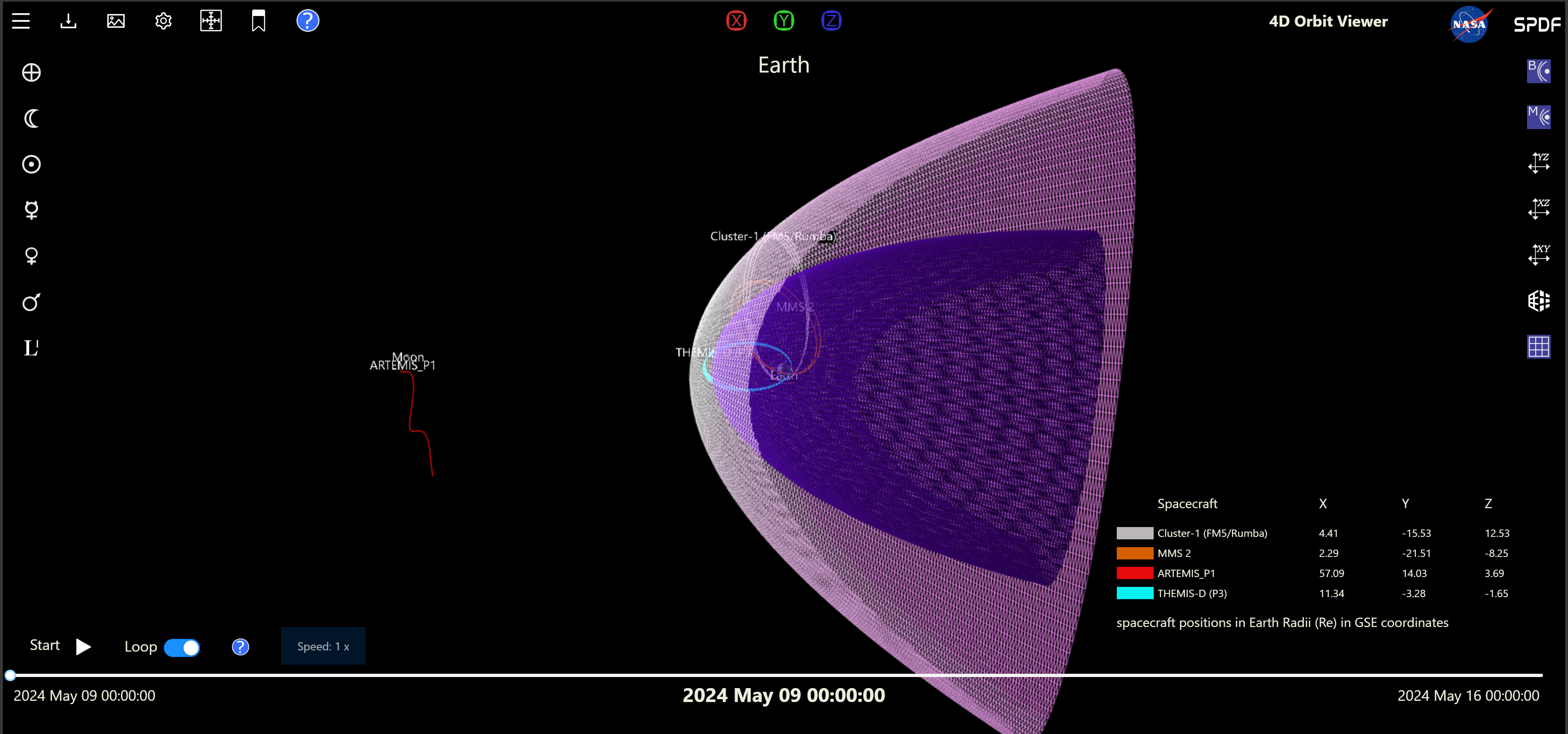
Figure 3. 4-D Orbit Viewer.
3. Generation of Text Listing Examples
Generation of text listings from SSCWeb can be produced from the Spacecraft Locator module, the Spacecraft Conjunction Query module, and the Coordinate Calculator module. Examples of each are included below.
This interface will output a human readable text list or a cdf file. It is a similar interface to Locator Graphics except it requires that the user specify options such as the desired coordinate system; these are found under the ‘Output Options’ button on the Command Menu. Located under the Command Menu box, x, y, z, lat, lon, and local time outputs can be in GEI/TOD, GEI/J2000, GEO, GM, GSE, GSM or SM coordinate systems. Additional output options are:
- Regions (for the s/c position, the magnetospheric regions and what regions would be intercepted by a radial line or field-line trace)
- Values (s/c radial distance from Earth, the B field strength, L-value and Invariant Latitude)
- Distance (s/c distance from modeled regions of the magnetosphere and the GSE X, Y, and Z components of the B field at the s/c)
- B field trace (footprint latitude and longitude, arc length) regions, values, and distance, and B field trace output options
Time and units output formats can also be customized. The Advanced interface enables filtering of the satellite position based on the Regions, Values and Distances described above as well as adjusting the B field models and their input parameter values.
Listing Example 1
Enter the following selections to produce Figure 4:
- Satellites: RBSP-A and B
- Time Range: 2018/05/23 12:30 to 2018/05/23 12:37
- Output Options:
- Coordinates: X,Y, Z in GSM
- Regions: Spacecraft Regions
- Values: Radial distance
- Output Units/Formatting: Date: yy/mm/dd
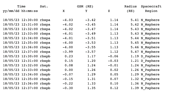
Figure 4. Locator Tabular Output.
This is a more complex interface. The user can select one or more spacecrafts for the two query options:
- Region Filters: User has choices of Spacecraft Regions, Radial Trace Regions, and Magnetic Map
- Regions: Output will be a human readable list of start/stop times when one or more of the spacecrafts selected cross in/out the selected regions
Listing Example 2
Enter the following selections to produce Figure 5:
- Spacecrafts: Cluster 1 through 4
- Dates/times: 2019/07/19 00:00 to2019/07/19 10:20
- S/c Regions: Select All
- Date format: yy/mm/dd

Figure 5. Output of Regions.
Conjunction Conditions
There are two conjunction queries:
- The Ground Station option will return a list of human readable times when one or more spacecrafts cross an area where the magnetic field line traces down to the selected ground stations. (Snapshot of output)
- The Lead Satellite option will provide a list of human readable times when one or more spacecrafts occupy the same magnetic flux tube of force as the selected lead satellite
Listing Example 3
Enter the following selections to produce Figure 6:
- Spacecrafts: Fast, THEMIS A through E
- Dates/times: 2008/2 14:00 to 2008/2 17:59:59
- Lead sat: fast

Figure 6. Output of Lead Satellite.
The Coordinate Calculator is a simple interface where the user inputs a date and time, and a point in space in cartesian (x, y, z) coordinates in GEI, GEIJ2000, GSE, GSM or SM, or spherical coordinates (lat, lon, radius) in GEO or GM. The calculator will output that point in all other coordinate systems and the B-trace of the point’s position in the magnetosphere.
Listing Example 4
Enter the following selections to produce Figure 7:
- Date/Time: 2020/85 10:00
- Input coordinate: GEI
- Values: x=2, y=1.5, z=0.5

Figure 7. Output of Coordinate Calculator.
4. Web Services Discussion and Examples
One of the newer SSC capabilities, the Web Services, allow user-written programs to retrieve any spacecraft ephemeris and other outputs contained in the SSC system without the use of the web pages, using HTTPS and supporting REST and SOAP styles network transport services.
Web services are best utilized by software developers comfortable working in C/C++, Java, Javascript, IDL or Python.
The simplest example of a RESTful application is the use of the ‘curl’ unix command:
$ curl -s https://sscweb.gsfc.nasa.gov/WS/sscr/2/observatories | xmllint —format -
If the user’s system can run ‘curl’ and ‘xmllint’, copy and paste this line to the terminal window to see an XML formatted list of all spacecrafts available on SSC together with
their respective time resolution, start and stop times when data is available, and other identifiers if these are available.
The ‘observatories’ part of the above URL can be changed in order to retrieve other desired information.
See https://sscweb.gsfc.nasa.gov/WebServices/REST/ for an extensive list and further examples.
For Python and non-Python programmers alike, the SSCWS Example Jupyter Notebook
offers helpful examples of using the SSC Web Services in a Jupyter Notebook environment.
