An official website of the United States government
Here's how you know
Official websites use .gov A
.gov website belongs to an official government
organization in the United States.
Secure .gov websites use HTTPS A
lock (
) or https:// means you've safely connected to
the .gov website. Share sensitive information only on official,
secure websites.
This center is an operational unit of the Space Physics Data Facility SPDF and previously the National Space Science Data
Center’s NSSDC international counterpart, World Data Center A for Rockets and Satellites (WDC-A-R&S). SSC personnel and software
systems support NASA and international space physics activities by maintaining an ephemeris database for scientific satellites
in geocentric or heliocentric orbits which can be used to plan and support analysis of coordinated science observations by multiple
satellites. The SPDF provides software development and operational support for SSC; they are part of the Heliophysics Science Division at NASA Goddard Space Flight Center.
The SSC was established in the mid-1970’s to support and coordinate multi-mission planning for the International Magnetospheric
Study (IMS) [Teague et al., 1982]. SSC software resources developed during the IMS era continued to be used in mission and science
planning for missions such as Dynamics Explorer 1 and 2 (DE 1/2), the International Sun-Earth Explorer series (ISEE 1, 2, and 3),
and the Interplanetary Monitoring Platform series (IMP 7 and 8). The SSC supported the ongoing series of Coordinated Data Analysis
Workshop studies that began in 1978. In 1986 SSC played a major planning and coordination role during the multi-mission Polar Region
and Outer Magnetospheric International Studies (PROMIS) program. Later SSC similarly supported the Solar Terrestrial Energy Program
(STEP) during 1990-1994. Additional projects that continue to be supported by SSC are NASA’s Global Geospace Science (GGS) program, the International Solar Terrestrial Physics ISTP , and the International Heliospheric Study (IHS).
Updated orbital elements for many active satellites are routinely received electronically by SSC from the United States Space Command (USSPACECOM/USSTRATCOM), previously known as NORAD. Elements for active satellites of interest to NASA-supported missions and international programs are processed by SSC staff into time-ordered Cartesian (X-Y-Z) coordinates, and stored in a database within the SSC Software System in SPDF/NSSDC’s Common Data Format CDF [Treinish and Gough, 1987]. The Cartesian data points are stored at maximum time resolution of one minute in Geocentric Equatorial Inertial True of Date (GEI TOD) coordinates. SSC originally used software maintained at NASA Goddard’s Flight Dynamics Division, and now uses open source software for processing Two-Line Elements (TLE) from Space-Track.org, and the NASA NIAF SPICE library for processing the orbit kernels from many active missions. SSC also pulls orbit data directly from other active missions.
The software and hardware capabilities of SSC have evolved over many years since the first generation of SSC programs was written in FORTRAN to run on a MODCOMP IV/25 computer for production of simple reports and data listings. In 1975, an interactive graphics system was added for preconfigured plots of key orbital parameters. In 1985, the software was ported to a MODCOMP Classic II/45 computer after previous updates and additions in 1980 in support of the Dynamics Explorer mission. Upgrades have included ports to more powerful computers in the SUN/UNIX environments and most recently (September, 2011) the operational system was ported to the Linux environment. In addition, upgrades have been made to the magnetic field models [Peredo et al., 1992] and the definitions for magnetospheric regions. Whereas user queries were exclusively handled by SSC staff prior to spring 1993, the emergence of the SSC Software System into the NSI network environment now makes possible direct access to SSC software and data by the space science community. The latest development in this area has been the creation of a web interface to the SSC. Users can access the Graphical User Interface of their browser to access the SSC database.
1.2 SSCWeb Software System
The SSC Software System is based on models of the Earth’s magnetospheric regions and magnetic field, and programs generate information listings and trajectory plots for purposes of planning spacecraft instrument operations and/or data analysis. These programs identify the time periods during which a specified spacecraft is in a particular magnetospheric region or is in magnetic conjunction with other spacecraft or ground stations; allow a choice of internal and external magnetic field models for field-line tracing options (Internal, IGRF; External, Tsyganenko); plot spacecraft trajectories, illustrating spacecraft position relative to various magnetospheric regions; and perform conversions among geocentric and magnetic coordinate systems.
An easy-to-use web interface allows the user to quickly move from one part of the system to another, and to easily specify input parameters and options. The SSC software provides the user three options for querying and viewing data available in an extensive database. These options, Query, Locator, and the database itself are described in the following sections.
The main section of this guide is organized to match the items presented to the user by the SSCWeb interface. Technical descriptions of the magnetic field models, magnetospheric region definitions, and coordinate systems used, as well as a list of usable ground stations, are given in Appendices A, B, C and D, respectively. Appendix E contains a glossary of terms used throughout the system itself and the documentation. User comments, suggestions and problem reports can be sent to: gsfc-spdf-support@lists.nasa.gov.
1.3 Locator
The Locator component of the SSC system allows the user to obtain location data in a tabular format. The user may request the spacecraft’s location converted into a variety of coordinate systems as well as the following coordinate related items:
Latitude and longitude values of magnetic field line traces from the spacecraft location
The magnetospheric region in which the spacecraft resides
Radial distances from the Earth’s center to the spacecraft (in Km or in RE, where RE=6378.16 Km)
Distances from the spacecraft to the:
Bow shock
Magnetopause
Tsyganenko 95 neutral sheet
The spacecraft’s corresponding:
L value
Magnetic field strength
Invariant latitude
1.4 Query
The Query processor provides two query matching options, magnetospheric region occupancy and magnetic field line tracing. The region setup option provides magnetospheric region occupancy by listing the entry and exit times in which specified satellite(s) were in particular magnetospheric regions. The trace setup option provides the means to perform field line tracing queries to identify either periods when one or more spacecraft are on the same magnetic flux tube of force as a specified lead spacecraft, or periods when one or more spacecraft occupy a field line which traces down to a specified ground station.
At intervals equal to the time between successive ephemeris data points, the ephemeris information of each spacecraft is used to evaluate the magnetic field vector at the position of the spacecraft. Next, the sampling point is moved in the direction of the vector to reach a neighboring point along the tube where the local field vector specifies the direction of the next step. This process is then iterated until finally the footpoint of the tube is reached. The magnetospheric models available for field line tracing are listed in Appendix A.
To facilitate complex queries, the user can specify up to nine conditions under which a single query may be made. A condition consists of satellite selections, region specifications, and field line tracing options. PLEASE NOTE that the condition number is located at the top of the screen. The trace model selection, as well as the start and stop times, are used throughout all conditions.
The main screen of the Query Interface requires selection of at least one satellite for processing from a scrolling list of available satellites, and entry of the start and stop times for satellite processing.
Query also contains fields for specifying whether the satellites, time ranges and setups will apply to the current condition, to all of the conditions, or to any of the conditions. These conditions may be queried independently, or together.
Several models are available to independently specify the terrestrial (internal) magnetic field and the magnetospheric (external) magnetic field. The size of the magnetic flux tube can also be specified as either a bin of x-deg latitude by y-deg longitude or a circular tube of a specified radius.
1.5 Extensive Database
Extensive Database
Updated predictive and definitive ephemeris for over 150 satellites are maintained at the SSC. Time and position over specific time periods at varying resolutions are stored for each satellite. The orbital elements themselves are not currently stored in the database. This database is updated periodically with ephemeris for new satellites or revised ephemeris for existing satellites.
1.6 Navigation Help for SSCWeb
The information below will help users effectively to navigate through the SSCWeb.
DO NOT USE the browser’s back and forward commands. The proper way to navigate these pages is to utilize the command menu located at the bottom of each page. As you enter information and move from page to page the information is stored in “hidden” fields that are part of the document but not displayed. Using the back and forward command supplied by your browser will result in these hidden fields not being updated and your input will be lost and/or your results incorrect.
Selecting multiple items in a scrolling list varies depending on the platform.
On Macintosh:
Holding down the Shift key will select everything between the item selected and the previous item selected.
Holding down the Command key will allow you to select several items that are not adjacent to one another.
On Windows:
Holding down the Shift key will select everything between the item selected and the previous item selected.
Holding down the Control key will allow you to select several items that are not adjacent to one another.
On Unix:
Select multiple items by selecting them one at a time.
Using the Help Window
It is best to use a frames enabled version of a browser. With frames there will be a small portion of the screen where help text will be displayed. You will be able to get help on any item that is marked as a link on the SSCWeb Form. Please be aware of the following to make using help easier:
You can modify the size of the help window by “grabbing” the bar between the frames and moving it in the desired direction.
Using the browser’s “Back” command has different results from browser to browser and even between the same browser on different platforms.
If you switch to the ADVANCED interface your input from the STANDARD interface will still be valid. Any options you selected in ADVANCED interface will still apply to any query you submit but will not be editable from the STANDARD interface.
2.0 Tutorial
2.1 Starting Out
SSCWeb allows users to move easily from one part of the system to another while specifying input parameters and options. The left side has a menu of SSC services, tutorials, and additional services to help the user become familiar with SSCWeb. The middle of the page has announcements, links to database contents, and SSCWeb’s graphics and listing services. The Spacecraft Availability and Time Ranges link takes the user to a page that lists all of SSC holdings. The user can use this list to help chose a spacecraft and start and stop times for a data request. Data Provenance provides detailed mission information including status, frequency of data updates, and data origination. This document will focus on two services SSC provides: Graphics and Listing outputs. Figure 1 below shows a part of the home page.
Figure 1. SSCWeb Home Page.
2.2 Navigation
The SSCWeb contains two components, Graphics and Listings. Graphics contains two sub-components- Locator Graphics and 4-D Orbit Viewer. Listings contains three sub-components- Locator Tabular, Query, and Coordinate Calculator. Locator Graphics, Locator Tabular, and Query have both Standard and Advanced interface options for users to choose. There are several differences between the Standard and Advanced interfaces. The changes revolve around the Command Menu and the number of options that are available for filtering.
Above the Graphics section there is a link for ‘Spacecraft Availability & Time Ranges.’ This page allows the user to browse available satellite ephemerides. The database includes the name of the satellite, the time resolution of the data in seconds, time range of available data, and whether the data is predictive or definitive.
2.3 Graphics
2.3.1 Locator Graphics
The Locator graphics component provides the ability to plot the orbits of multiple spacecraft. In addition to orbit plots, mapped and time series plots can also be generated. Select one or more satellites (use CMD-left_click or SHIFT-left_click for multiple selections) and a plot type. Type in a time range in any of the valid formats and select Plot. Any warnings or errors will be at the top of the page displayed. If there are no errors, the requested plot is displayed together with a PS and PDF plot option to download. To make a new request or add options to the current plot scroll down to the Command Menu at the bottom of the page and make selections.
Figure 2. SSCWeb Locator Graphics Form.
2.3.2 4-D Orbit Viewer
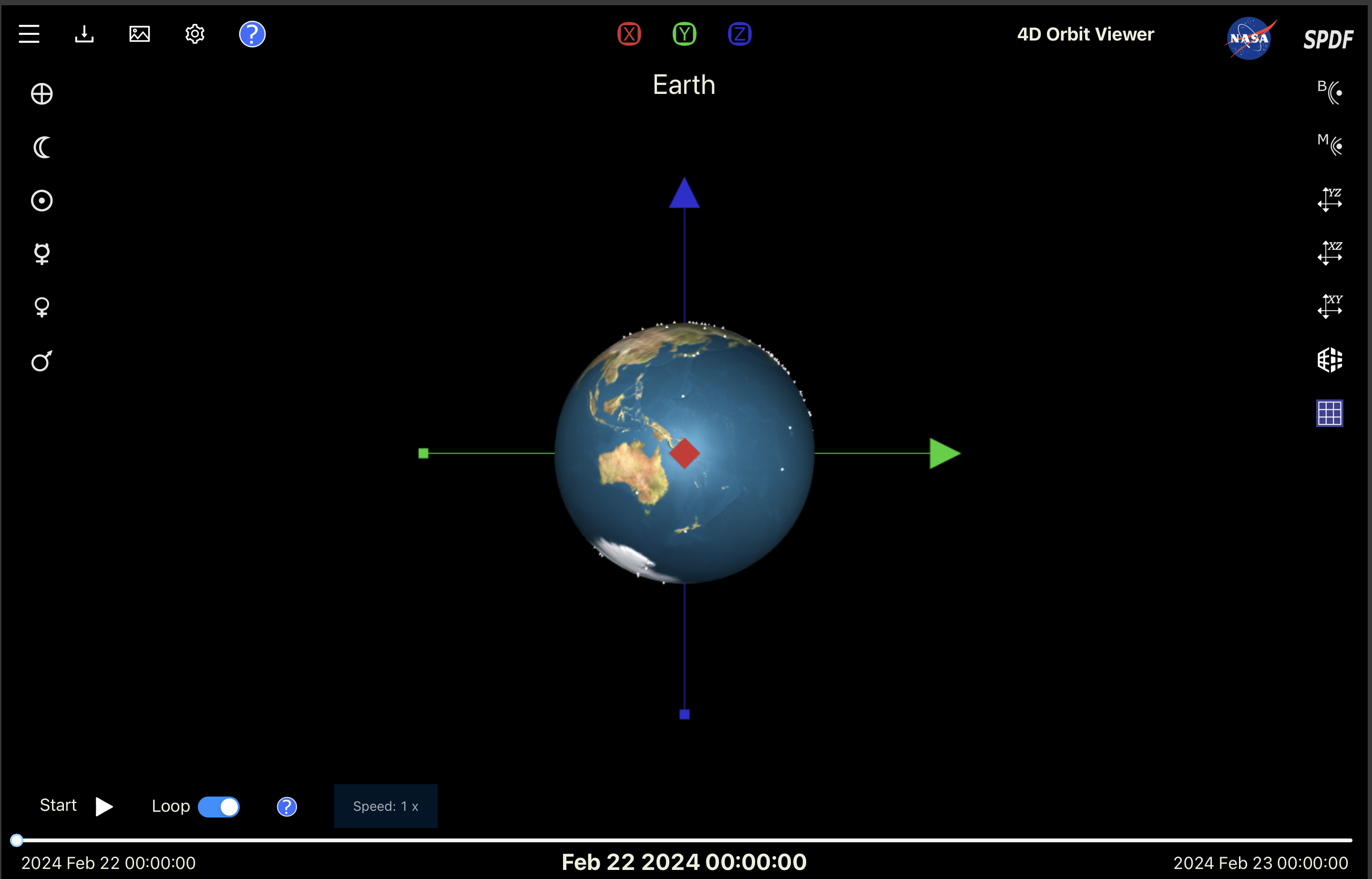
This application provides the user with the capability to select spacecraft(s) and time ranges of interest, and see their orbits represented as an interactive 4-D animation. The locations and orbits of over 100 spacecraft and planets stored in the SSC are viewable in the SPDF 4-D Orbit Viewer as an interactive 3-D animation with time as the 4th dimension. A prototype browser-based tool is now available to replace the original Java-based tool. Trajectories are displayed in a virtual 3-D environment which also includes the four inner planets (Mercury, Venus, Earth, and Mars) and the Sun and Moon (Luna). More detailed help is available either by hovering over interface elements to reveal tool tips specific to that control or by clicking on the question mark icon, which appears in various parts of the interface and will bring up detailed instructions related to that part of the program.
Figure 3. SSCWeb 4D Orbit Viewer.
2.4 Locator Tabular
The Locator component provides tabular information. As tabular output, the spacecraft’s location can be listed in a variety of coordinate systems, as well as other location related items.
Figure 4. SSCWeb Locator Tabular Form.
At the heart of the Tabular Output system is the “Command Menu” which is displayed at the bottom of every screen. Users should be aware that the “Command Menu” should be their primary means of navigating through the Locator Tabular Ouput portion of the Satellite Situation Center.
2.4.1 Standard Interface
As pictured in Figure 4 above, the Command Menu is divided into four areas. The numbers beside each of the first three areas are intended to provide the user with a reminder of the order in which these options should be accessed. Each option will be described in detail in the following sections.
Command Menu 1: REQUIRED SETTINGS Output Options
Standard Interface Output Options Screen
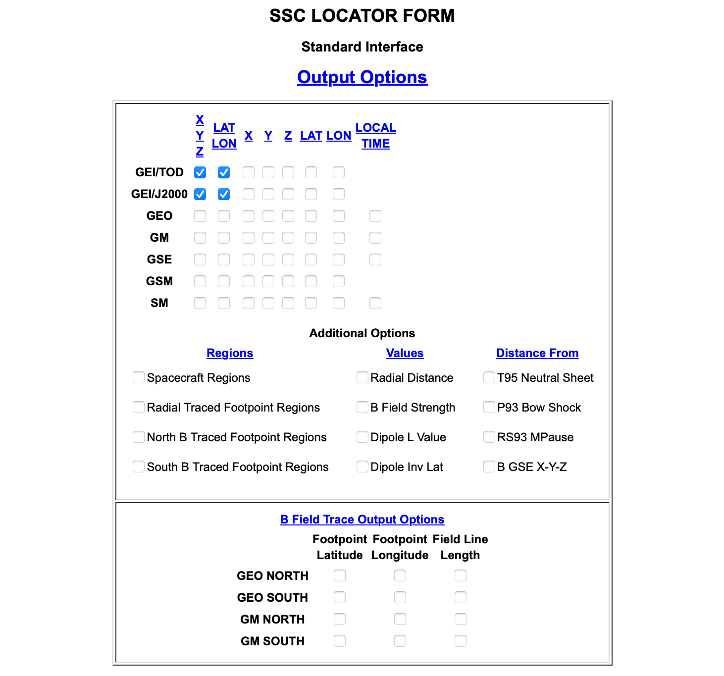
The user has many options on this screen, as shown in Figure 5 below. Regions, values, distances, coordinate systems, and B field trace options are available. On the left hand side are the available coordinate systems that the software can present the ephemeris data.
The selection for output of GEO and/or GM coordinates of magnetic field line footpoints in either magnetic hemisphere (i.e. resulting from a north or south magnetic field line trace) may be obtained by selecting the appropriate checkboxes at the bottom of the screen. The field line in question is that which passes through a spacecraft at a given point in time. In addition to field line footpoints, the arc length of the line from the spacecraft to either footpoint can also be obtained. The next sections are optional and deal with reducing the output by filtering on values that will be output by the software as well as the format of the output.
Figure 5. Standard Interface Output Options.
Command menu 1: OPTIONAL SETTINGS Output Units/Formatting
The Output Units/Formatting screen allows the user to select the format for the outputs for date, time, distance, degrees, and direction/range. In addition the user can select the number of lines per page. The default value of 1 will produce one header for each column instead of every XX number of lines. If the user enters a 0 in this field the output will have no column headers. The user may also select to output the information into a CDF file. This will create as CDF file in the public FTP area. The user may then download this file.
Standard Interface Output/Formatting Screen
The bottom line of the command menu contains a pair of buttons labeled “Interface Style: Standard Advanced.” The button is defaulted to the Standard button. However, at any time the user can select the Advanced button and when the next page is loaded the advanced interface will be shown.
Command menu 2: Input Summary
The Input Summary option on the Query Processor Main Menu screen allows users to view their selections prior to executing a query. An output summary is available for both screen and file outputs. File output summaries precede the actual output within the same file.
Command menu 3: EXECUTION OPTIONS
The Execute button will execute the query. Besides the ‘Plot’ button for Graphics and the ‘Submit query and wait for output’ button for Tabular, the SSCWeb also provides an option to ‘Prepare query to be saved locally.’ This option saves the state of the page and all the user selected options so that a user can return to the page at a later time.
2.4.2 Advanced Interface
There are now several more choices under “Optional Settings.” These additional choices provide several filtering options. The filtering options are expanded to allow the user to filter any of the available output parameters whether or not that parameter is included in the output.
Filtering Options
If the user selects “Filtering Options” the Advanced Interface Filtering Options screen will be displayed.
Advanced Interface Spacecraft/Time Range Selection Screen
The user can specify a “Database Resolution Factor” for each spacecraft that is selected. They can also filter based on any of the available coordinate systems as opposed to only those selected for output in the Standard Interface.
Command Menu 1: REQUIRED SETTINGS Output Options
The output options are the same in the Advanced Interface as they are in the Standard Interface.
Regions Filter
At the bottom of the screen there may be one or more “Region Filters” depending on what was selected on the “Output Options” screen.”Regions” denotes a naming convention of three dimensional and two dimensional zones that are associated with a spacecraft’s location for a particular point in time. The “Regions Filter” section of the screen displays the four types of regions that can be generated. The specific regions that constitute each region type are listed below. When in the ‘Regions Filter’ screen, a selection of a region type will display a selectable list of the regions specific to that region type.
Selecting specific regions will constrain the displayed results to spacecraft locations that are in at least one of those selected regions for a particular region type. If the request “meet ‘ALL’ region filters” has been made, then the displayed results will be constrained to spacecraft locations that are in at least one of the selected regions OF EACH REGION TYPE for which specific regions have been specified.
SPACECRAFT REGIONS- (3 dimensional zones) Such a region is based on the spacecraft’s position. A spacecraft can occupy only one region of this region type at any given time. A spacecraft region assignment can be one of the following:
Interplanetary medium
Dayside Magnetosheath, Nightside Magnetosheath
Dayside Magnetosphere, Nightside Magnetosphere
Dayside Plasmasphere, Nightside Plasmasphere
Plasma Sheet
Tail Lobe
LLBL (Low Latitude Boundry Layer)
HLBL (High Latitude Boundry Layer- formerly known as the Mantle)
RADIAL TRACED FOOTPOINT REGIONS- (2 dimensional zones) such a region is based on the location on the Earth’s surface where a straight line would intersect when connecting the spacecraft and the Earth’s center. A radial traced region assignment can be one of the following:
North Polar Cap, South polar Cap
North Cusp, South Cusp
North Cleft, South Cleft
North Auroral Oval, South Auroral Oval
North Mid-Latitude, South Mid-Latitude
Low Latitude
Note: The North and South Mid-Latitude regions are defined as the two bands about the Earth that extend from: +30 degrees latitude to the North Auroral Oval, and -30 degrees latitude to the South Auroral Oval. The Low-Latitude is the band that extends from +30 degrees latitude to -30 degrees latitude.
NORTH B TRACED FOOTPOINT REGIONS- (2 dimensional zones) such a region is based on where the magnetic field line that passes through the spacecraft intersects the Earth’s surface in the Earth’s northern magnetic hemisphere. North B traced footpoint region assignments are the same as the ‘North’ regions and the Low Latitude region used for assigning a radial traced footpoint region.
SOUTH B TRACED FOOTPOINT REGIONS- (2 dimensional zones) such a region is based on where the magnetic field line that passes through the spacecraft intersects the Earth’s surface in the Earth’s southern magnetic hemisphere. South B traced footpoint region assignments are the same as the ‘South’ regions and the Low Latitude region used for assigning a radial traced footpoint region.
Command menu 1: OPTIONAL SETTINGS
These additional options are an expansion of the available filtering options.
Spacecraft location filters
Spacecraft region filters
Additional locations filters
B field model selection
Output units/formatting
Command menu 2: Input Summary
The Input Summary options are the same in the Advanced Interface as they are in the Standard Interface.
Command menu 3: EXECUTION OPTIONS
The Execute button will execute the query.
2.5 Query
The Query component provides two query matching options: magnetospheric region occupancy and magnetic field line tracing. The user can specify up to nine conditions under which a single query may be made. A condition consists of satellite selections, region specifications, and field line tracing options.The example here is for region specifications. The region query lists the entry and exit times during which specified satellite(s) were in particular magnetospheric regions. The trace query identifies periods when one or more spacecraft are on the same magnetic flux tube of force, or periods when one or more spacecraft occupy a field line which traces down to a specified ground station. The current condition number and the total number of conditions entered is located at the top of the command menu. The trace model selection, as well as the start and stop times, are used throughout all conditions.
The first screen of the Query Interface requires selection of at least one satellite for processing from a scrolling list of available satellites, selection of whether all the satellites or any number of them must meet the conditions to be specified, and entry of the start and stop times for satellite processing.
Figure 6. SSCWeb Query Form.
2.5.1 Standard Interface
Command Menu: Query Parameters
The Query Parameters Screen displays the primary fields for specify the query criteria. At the top of the screen there are two choices to identify which magnetospheric regions the satellites must occupy for inclusion in output processing. Alternatively, the user may choose to ignore the regions. This is useful if trace criteria have been entered and region criteria are to be ignored for the current condition. Multiple condition queries can be executed by using the Advanced option.
Meet ALL Region Filter groups (AND)
Each satellite must be in the same selected region to be included in the output.
Meet ANY Region Filter groups (ANY)
The satellite(s) may be in any of the selected regions to provide a conjunction.
Ignore Region Groups
Region query testing is not performed. Once the Same or Any option is determined, one or more magnetospheric regions must be selected.
Command Menu: Output Formatting
The Output Units/Formatting screen allows the user to select the format for the outputs for date, time, distance, degrees, and direction/range.
Command menu: Input Summary
The Input Summary option on the Query Processor Main Menu screen allows users to view their selections prior to executing a query. An output summary is available for both screen and file outputs. File output summaries precede the actual output within the same file.
Command menu: Execution Options
The Execute button will execute the query. While the output is being processed a window will display the percentage of processing currently completed.
2.5.2 Advanced Interface
The Advanced Interface allows the user to select a combination of conditions.
Command Menu: Required Input
Occupancy/Conjunction Condition Combinations, and region, ground station or lead satellite
Command menu: Optional Input
Edit/add ground station info
B field model selection
Command Menu: Output Formatting
The Output Units/Formatting screen allows the user to select the format for the outputs for date, time, distance, degrees, and direction/range.
Command menu: Input Summary
The Input Summary option on the Query Processor Main Menu screen allows users to view their selections prior to executing a query. An output summary is available for both screen and file outputs. File output summaries precede the actual output within the same file.
Command menu: Execution Options
The Execute button will execute the query. While the output is being processed a window will display the percentage of processing currently completed.
Region Selection
This option is located beneath the region occupancy field. This area displays the magnetospheric regions and mapped regions available for satellite occupancy testing. Mapped regions are subregions which correspond to areas on the Earth’s surface into which field lines from the satellite’s orbital position traces. The Trace Setup fields are located at the bottom of the screen. The Trace Setup option is a series of pull-down menus for selecting conjunction conditions, trace direction, B-field model, and output format. Regardless of the conjunction condition, specify the trace direction or hemisphere as either down to the same hemisphere as the satellite, either/both hemispheres, opposite hemisphere, northern hemisphere or southern hemisphere.
2.6 Coordinate Calculator
In order to use Coordinate Calculator, enter the date and time in the format indicated, then the coordinates in either Cartesian or Spherical system, in the units indicated. Lastly, identify the coordinate system of the inputs. The output is the radial distance of the spacecraft; a list of values indicating spacecraft position in all coordinate systems listed on the front page, in both Cartesian and Spherical systems, and the local time if applicable; and the region of space occupied by the spacecraft. Additionally, the user will see a list of B-trace outputs. This list includes the default magnetic field models utilized; the radial distance of the spacecraft in Re units; a list of Lat, Lon and trace values in GEO and GM coordinates; the B Total value and radial, theta and phi components; and regions mapped on Earth by the North and South traces and Radial position of the spacecraft.
Figure 7. SSCWeb Coordinate Calculator.
Appendix A: Magnetic Field Models in the Satellite Situation Center Software
Currently the SSCWeb carries three magnetic field models for the external currents, besides the lower altitude IGRFs:
Model
Database s/c
Activity Levels
Tailward range of validity
Comments
T87Wd
IMP,HEOS,ISEE
6 Kp
70 RE
Warped neutral sheet
T89c
IMP,HEOS,ISEE
7 Kp
70 RE
Revised T89, with more data
T96
IMP,HEOS,ISEE
7 Kp
70 RE
Bz, By, Dst
The original datasets are almost identical in all three above models. The data were gathered from several s/c as listed below.
Spacecraft
Time Interval Used
No. Points
Total Time,hours
No. Orbits
A-IMP D (Explorer 33)
July ‘66 - July ‘68
724
356
34
A-IMP E (Explorer 35)
July ‘67 - Jan ‘69
1,260
1,260
17
IMP 4 (IMP F, Explorer 34)
May ‘67 - Sept ‘71
5,173
2,799
144
IMP 5 (IMP G,Explorer 41)
June ‘69 -Sept ‘71
9,426
5,480
195
IMP 6 (IMP I, Explorer 43)
Mar ‘71 - Sept ‘74
11,801
5,419
312
HEOS 1
Dec ‘68 - Dec ‘73
3,908
1,980
215
HEOS 2
Feb ‘72 - Aug ‘74
3,044
1,320
152
IMP 7 (IMP H, Explorer 47)
Sept ‘72 - Apr ‘73
681
650
14
IMP 8 (IMP J,Explorer 50)
Oct ‘73 - June ‘86
9,568
8,052
280
ISEE 1
Jan ‘80 - Dec ‘81
17,602
6,794
301
ISEE 2
Jan ‘78 - Jan ‘80
16,558
6,497
311
Totals
79,745
40,607
For additional information about these data sets please refer to “A large magnetosphere magnetic field database,” Fairfield et al. JGR, 99, 11319, 1994.
Appendix B: Models and Regions of Geospace in the Satellite Situation Center Software, V. 2.2
As part of the modernization of the magnetic field models and geospace region definitions used in the Satellite Situation Center (SSC) software, a radical change was introduced between Versions 2.1 and 2.2 in terms of the philosophy used to define regions of geospace. Versions 2.1 and earlier essentially employed a single “index” to identify regions, without distinction between regions in space and regions on the ionosphere (or ground). Version 2.2, in contrast, involves multiple indices to specifically differentiate the region in geospace that the satellite resides in, and the (mapped) regions on the ionosphere (or ground) that the subsatellite point or magnetic footpoint(s) fall in. Thus, the new geospace region definitions involve a family of “spacecraft regions,” and a family of “mapped regions,” as listed below:
Regions of Geospace
Spacecraft Regions:
Spacecraft Region
Code recorded when output = CDF
None
0
Interplanetary Medium
1
Dayside Magnetosheath
2
Nightside Magnetosheath
3
Dayside Magnetosphere
4
Nightside Magnetosphere
5
Plasma Sheet
6
Tail Lobe
7
High Latitude Boundary Layer
8
Low Latitude Boundary Layer
9
Dayside Plasmasphere
10
Nightside Plasmasphere
11
Mapped Regions:
Mapped Region
Code recorded when output = CDF
None
0
Northern Cusp
1
Southern Cusp
2
Northern Cleft
3
Southern Cleft
4
Northern Auroral Oval
5
Southern Auroral Oval
6
Northern Polar Cap
7
Southern Polar Cap
8
Northern Mid-latitude
9
Southern Mid-latitude
10
Low-latitude
11
Users may request, independently, information on any of the four region identifier indices: 1) spacecraft region, 2) radially mapped region (i.e. the subsatellite point), 3) northern magnetic footprint region, 4) southern magnetic footprint region. Magnetic field traces are performed using a user-selectable combination of internal and external magnetic field models.
Regions and Boundaries in the SSC Software: Algorithms
Spacecraft Regions:
The Interplanetary Medium, Magnetosheath, and Magnetosphere regions are defined by model boundaries for the magnetopause and bow shock surfaces.
For the Magnetopause, the Roelof and Sibeck model (JGR, 98, 21421, 1993 ) is employed. The model represents the boundary as a “quadratic function” in aberrated GSE coordinates; namely:
R2+S1X2+S2X+S3=0R2=Y2+Z2
where S1, S2 and S3 are functions of the solar wind dynamic pressure Psw and the IMF-Bz component
For the Bow Shock, a Modified version of Fairfield’s 1971 model (JGR, 76, 6700, 1971) arranged to move in and out in response to solar wind and IMF changes, in unison with the magnetopause, and constrained to fixed ratio between the subsolar distances to the bow shock and magnetopause, Rbs/Rmp=1.3
R2+A(X−X0)R+B(X−X0)2+CR+D(X−X0)+E=0R2=Y2+Z2
The Neutral Sheet definition is based on the current sheet model used in new Tsyganenko models (JGR, 100, 5599, 1995). The current sheet surface is described by the equation:
where (x,y, z) are aberrated GSM coordinates, psi is the tilt angle, and the “scaling” parameters are set to: Rh = 8, d = 4, G=10, Ly = 10
The Plasma Sheet model, as labelled in the SSC, is meant to include both the plasma sheet (PS) and plasma sheet boundary layer (PSBL) since no community-accepted models exist (as far as we know) to represent these regions independently. The PS region is thus defined as a strip extending 3 Re above and below current sheet surface.
The High Latitude Boundary Layer (HLBL) and Low Latitude Boundary Layer (LLBL) regions are defined in relation to the magnetopause and neutral sheet. Using GSM coordinates, an anular strip of thickness D = D(X) is defined inside magnetopause; D widens from 0.4 Re at the terminator to 4 Re at X=-40 Re, and is held fixed at 4 Re tailward of X=-40 Re. Points inside the strip and within 3 Re of the neutral sheet surface are labelled as LLBL, while those in the strip but more than 3 Re from the neutral sheet are tagged as HLBL.
The Tail Lobe region is defined as points tailward of the “hinging distance” (Rh = 8), inside the tail but not in PS, HLBL or LLBL.
The following diagram illustrates graphically the layout of the regions described above:
Figure 8. SSCWeb Regions Layout.
The Plasmapause is defined according to the model of Gallagher, et al., (Adv. Space Res. 8, 15, 1988) which represents the plasma density n as a function of the L-parameter, the magnetic local time (MLT) and the height, h, above the Earth’s surface. It can be seen in the equation below:
In the previous expression, lambda is the geomagnetic latitude. We define plasmapause as the surface give by log(n)=1.5 The region labelled Magnetosphere corresponds to points inside magnetopause but not in other s/c regions.
Mapped Regions:
The Cusp and Cleft regions are based on “statistical” description by Newell and Meng (JGR, 1988); namely, the Cusp is defined as the region MLAT= 75-76 degrees, MLT=09:00-13:00, while the Cleft is given by MLAT = 74-78 degrees, MLT=08:00-13:30.
The Auroral Oval boundaries AOHI and AOLOW are described by:
where C=22.5 degrees if MLT<22:50 and 337.5 degrees if MLT>22:50; S=+/-1 (nightside/dayside)
Finally, the Mid-latitude and Low-latitude regions are defined in terms of ranges in MLAT according to: Mid-lat from MLAT = 30 degrees up to the equatorward edge of auroral oval, and Low-lat by MLAT = -30 degrees to 30 degrees.
The various mapped regions are illustrated in the following sketch:
Figure 9. SSCWeb Mapped Regions.
Appendix C: Description of Selected Coordinate Systems Used in SSC Programs
GEI: Geocentric Equatorial Inertial system. This system has X-axis pointing from the Earth toward the first point of Aries (the position of the Sun at the vernal equinox). This direction is the intersection of the Earth’s equatorial plane and the ecliptic plane and thus the X-axis lies in both planes. The Z-axis is parallel to the rotation axis of the Earth, and y completes the right-handed orthogonal set (Y = Z * X). Geocentric Inertial (GCI) and Earth-Centered Inertial (ECI) are the same as GEI.
GEO: Geographic coordinate system. This system is defined so that its X-axis is in the Earth’s equatorial plane but is fixed with the rotation of the Earth so that it passes through the Greenwich meridian (0 longitude). Its Z-axis is parallel to the rotation axis of the Earth, and its Y-axis completes a right handed orthogonal set (Y = Z * X).
GM: Geomagnetic coordinate system. Z-axis points to the Geomagnetic north pole (in Greenland). The positive X-axis points towards the great circle encompassing the North and South Geomagetic poles and lies in the geomagnetic equatorial plane in the segment that is in the western hemisphere. (The South GM pole is the antipode of the North GM pole.) Earth-centered Dipole is invoked. Y completes the triad.
GSE: Geocentric Solar Ecliptic system. This has its X-axis pointing from the Earth toward the Sun and its Y-axis is chosen to be in the ecliptic plane pointing towards dusk (thus opposing planetary motion). Its Z-axis is parallel to the ecliptic pole. Relative to an inertial system this system has a yearly rotation.
GSM: Geocentric Solar Magnetospheric system. This has its X-axis from the Earth to the Sun. The Y-axis is defined to be perpendicular to the Earth’s magnetic dipole so that the X-Z plane contains the dipole axis. The positive Z-axis is chosen to be in the same sense as the northern magnetic pole. The difference between the GSM and GSE systems is simply a rotation about the X-axis.
SM: Solar Magnetic coordinates. In this system, the Z-axis is chosen parallel to the north magnetic pole and the Y-axis perpendicular to the Earth-Sun line towards dusk. The difference between this system and the GSM system is a rotation about the Y-axis. The amount of rotation is simply the dipole tilt angle. We note that in this system the X-axis does not point directly at the Sun. As with the GSM system, the SM system rotates with both a yearly and daily period with respect to inertial coordinates.
Invariant Latitude: For any point in space one can trace a B-field line to the Earth surface, assuming it is a centered dipole field. The GM latitude of this foot point is labelled as the Invariant Latitude along the entire field line. The dipole L-value is closely related to this invariant latitude; L=1/(Cos(Lat))^2, and physically connotes the distance (in Earth radii) of the “top of the field line” from Earth center.
J2000: Geocentric Equatorial Inertial for epoch J2000.0 (GEI2000), also known as Mean Equator and Mean Equinox of J2000.0 (Julian date 2451545.0 TT (Terrestrial Time), or 2000 January 1 noon TT, or 2000 January 1 11:59:27.816 TAI or 2000 January 1 11:58:55.816 UTC.) This system has X-axis aligned with the mean equinox for epoch J2000; Z-axis is parallel to the rotation axis of the Earth, and Y completes the right-handed orthogonal set.
Appendix D: Selected Ground Magnetic Stations
Station Name
Code
Latitude
Longitude
Alert
ALE
82.5
-62.5
Alma-Ata
AAA
43.2
76.9
Alta
ALT
68.9
22.96
Amderma
AMD
69.47
61.42
Anchorage
AMU
61.24
-149.87
Arctic Village
AVI
68.13
-145.57
Arkhangelsk
ARK
64.60
40.50
Ashkhabad
ASH
37.95
58.11
Back
BKC
57.68
-94.23
Baker Lake
BLC
64.33
-96.03
Barrow
BRW
71.30
-156.75
Boulder
BOU
40.14
-105.24
Cambridge Bay
CBB
69.20
-105.00
Cape Parry
CPY
70.17
-124.72
Cape Schmidt
CPS
68.92
-179.48
Cape Town
CTO
-33.95
18.47
College
CMO
64.85
-147.83
Contwoyto Lake
COW
65.73
-111.25
Dawson City
DWC
64.07
-139.42
Dixon Island
DIK
73.54
80.56
Dourbes
DOU
50.10
4.60
Eskdalemuir
ESK
55.32
-3.20
Eskimo Point
EKP
61.10
-94.07
Ferraz
FRZ
-62.08
-58.39
Fort Churchill
FCC
58.80
-94.10
Fort McMurray
FMM
56.73
-111.38
Fort Simpson
FSP
61.75
-121.23
Fort Smith
FSM
60.00
-112.00
Fort Yukon
FYU
66.57
-145.27
Fredericksburg
FRD
38.21
-77.37
Gillam
GIM
56.85
-94.42
Glenlea
GLL
49.60
-97.10
Godhavn
GDH
69.24
-53.52
Golden
GDN
39.75
-105.16
Guam
GUA
13.58
144.87
Halley Bay
HBA
-75.52
-26.60
Heiss Island
HIS
80.62
58.05
Honolulu
HON
21.32
-158.06
Hornsund
HRN
77.00
15.55
Huancayo
HUA
-12.05
-75.34
Husafell
HSF
64.67
-21.03
Inuvik
INK
68.25
-133.30
Iqaluit
IQA
63.80
-68.60
Irkutsk
IRT
52.46
104.04
Isafjordur
IFJ
66.08
-23.13
Island Lake
ISL
53.88
-94.68
Ivalo
IVA
68.60
27.48
Izvestia
IZV
75.9
82.7
Kakioka
KAK
36.23
140.19
Kaliningrad
KNG
54.70
20.62
Karaganda
KGD
49.82
73.08
Kautokeino
KAU
69.02
23.05
Kevo
KEV
69.76
27.01
Kiev
KIV
50.72
30.30
Kilpisjarvi
KIL
69.05
20.70
Kiruna
KIR
67.83
20.42
Kotelny
KOT
76.00
137.9
Leningrad
LNN
59.95
30.71
Lycksele
LYS
64.62
18.77
Lynn Lake
LYN
56.85
-101.07
Magadan
MGD
60.12
151.02
McMurdo
MCM
-77.85
166.70
Meanook
MEA
54.62
-112.33
Mizuho
MZH
-70.43
40.20
Moscow
MOS
55.48
37.31
Mould Bay
MBC
76.20
-119.40
Muonio
MUO
68.02
23.53
Murmansk
MMK
68.95
33.05
Narssarssuaq
NAQ
61.10
-45.20
Newport
NEW
48.26
-117.12
Nipawin
NIP
53.50
-103.70
Norilsk
NOK
69.40
88.10
Norman Wells
NOW
64.90
-125.50
Novokazalinsk
NKK
45.80
62.10
Novosibirsk
NVS
55.03
82.90
Nurmijarvi
NUR
60.51
24.66
Onagawa
ONW
38.43
141.47
Ottawa
OTT
45.40
-75.55
Oulu
OUL
65.10
25.85
Pello
PEL
66.90
24.08
Pinawa
PNW
50.2
-96.04
Podk. Tunguska
POD
61.60
90.00
Poste Baleine
PBQ
55.27
-77.75
Rabbit Lake
RBL
58.22
-103.67
Rankin Inlet
RIT
62.80
-92.33
Red Lake
RDL
50.90
-93.50
Resolute Bay
RES
74.70
-94.90
Sachs Harbor
SAH
72.00
-125.00
San Juan
SJG
18.38
-66.12
Siple
SPL
-76.0
-84.0
Sitka
SIT
57.05
-135.33
Sodankyla
SOD
67.37
26.65
Sondrestrom
STF
67.02
-50.72
Sopoch. Karga
SKG
71.9
82.1
Soroya
SOE
70.54
22.22
South Pole
SPA
-89.99
-13.32
St. Johns
STJ
47.59
-52.68
Sverdlovsk
SVD
56.73
61.07
Syowa
SYO
-69.01
39.59
Talkeetna
TLK
62.30
-150.10
Tashkent
TKT
41.33
69.62
Tbilisi
TFS
42.09
44.71
Thule/Qanaq
THL
77.48
-69.17
Tixie Bay
TIK
71.58
129.00
Tjornes
TJN
66.20
-17.12
Tomsk
TMK
56.47
84.93
Tromso
TRO
69.66
18.95
Tucson
TUC
32.25
-110.83
Uedinenie
UDN
77.5
82.30
Uppsala
UPP
59.80
17.60
Victoria
VIC
48.52
-123.42
Vize
VIZ
79.5
78.1
Weston
WES
42.38
-71.32
Yakutsk
YAK
62.02
129.72
Yellowknife
YKC
62.40
-114.50
Appendix E: Glossary
Active field- the currently highlighted field on a Screen in which input is accepted from the user or which presents the Command that will be performed if this Field is selected.
Button- see push button or radio button
Checkbox- a figure used to allow the user to make non-exclusive specifications.
Checklist- a possibly scrollable set of textual entries from which the user may make or remove non-exclusive (i.e., one or more) choices that are indicated by marks which appear beside the chosen entries.
Click- quickly press and release the mouse button.
Command- an order to the computer’s user interface to perform some action.
Field- any area of a Window in which an option may be selected, a parameter may be specified, or information may be displayed. These include a Checkbox, Checklist, Key in, Label, Multi-line Edit, Push Button, Radio Button, Slider, or Text Display.
Menu- a list of choices, among which the user selects desired choice(s), such as: button menu - a Menu of Push Buttons pop-up menu - a Menu of Items activated without a cue to its existence.
Menu option- one of the user selectable choices in a Menu.
Point- to use the mouse to reposition the cursor to the desired location on the screen.
Push button- a rectangular figure which allows the user to execute a Command. When a Push Button has three dots following its label, choosing it causes a new Window to be displayed.
Radio button- a figure used to allow the user to make an exclusive specification (or selection) from a group of two or more possibilities. Specifying or selecting a possibility in such a group automatically de-specifies or de-selects any other possibility in that group.
Satellites- a scrollable checklist of all the satellites available in the system database. At least one satellite must be selected from this checklist.
Select- a data entry field which indicates how many satellites must meet the query criteria, specifically whether ‘All’ of the selected satellites, or ‘Any’ particular satellites must meet the query criteria. If ‘Any’ is selected, the user must indicate exactly how many of the selected satellites must meet the criteria.
Text display- an area of a Window which displays multiple lines of read only text.
Time range- a start and stop time from which the query processor is to retrieve satellite ephemeris data must be entered. The processor will retrieve epoch data only from the time interval specified. These times apply globally to each condition. Each time consists of a year/day format optionally followed by an hour format. The default value for hours is zero. The formats are as follows:
Year/Day Formats- in each case the 19 is optional, 1992 Sep 21 or 1992/9/21 or 1992 265.
Hour Formats- the decimal hour may be as many digits as desired and the seconds are optional in the hour:minute:second format.
Teague, M. J., D. M. Sawyer, and J. I. Vette. “The Satellite Situation Center, in The IMS Source Book.” Guide to the International Magnetospheric Study Data Analysis, edited by C.T. Russell and D. J. Southwood, pp. 112-116, American Geophysical Union, Washington, D. C., 1982.